- What Is Linear Regression?
- The Cost Function
- Gradient Descent
- Putting It All Together
- Recap
Contents
Linear Regression In Pictures
I have been learning machine learning with Andrew Ng's excellent machine learning course on Coursera. This post covers Week 1 of the course.
You should read this post if week 1 went too fast for you. I cover the same stuff, but slowed down and with more images!
I'll talk about:
- what linear regression means
- cost functions
- gradient descent
These topics are the foundation for the rest of the course.
What is linear regression?
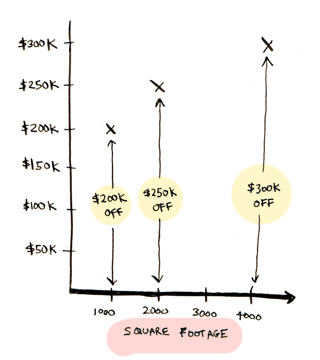
Suppose you are thinking of selling your home. Different sized homes around you have sold for different amounts:
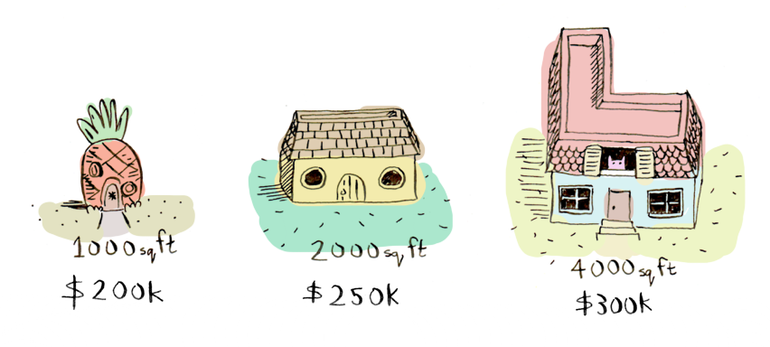
Your home is 3000 square feet. How much should you sell it for? You have to look at the existing data and predict a price for your home. This is called linear regression.
Here's an easy way to do it. Look at the data you have so far:
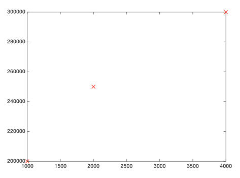
Each point represents one home. Now you can eyeball it and roughly draw a line that gets pretty close to all of these points:
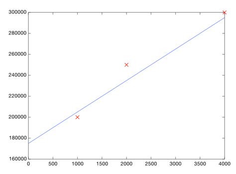
Then look at the price shown by the line, where the square footage is 3000:
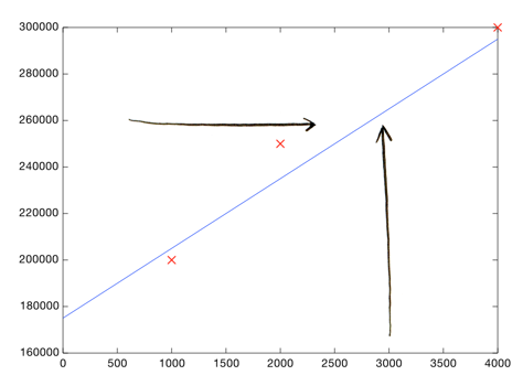
Boom! Your home should sell for $260,000.
That's all there is to it. You plot your data, eyeball a line, and use the line to make predictions. You need to make sure your line fits the data well:
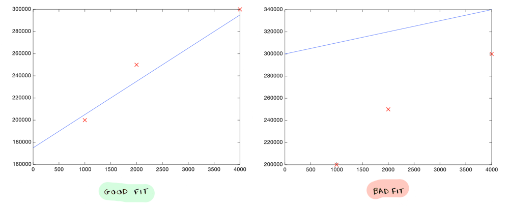
But of course we don't want to eyeball a line, we want to compute the exact line that best "fits" our data. That's where Andrew Ng and machine learning comes in.
How do you decide what line is good? Here's a bad line:
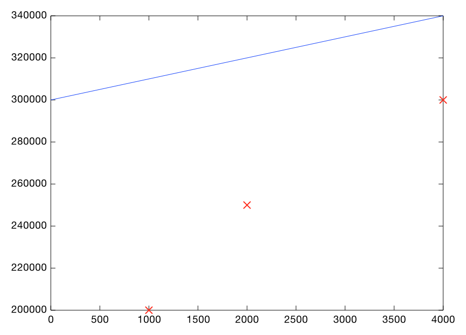
This line is way off. For example, according to this line, a 1000 sq foot house should sell for $310,000, whereas we know it actually sold for $200,000:
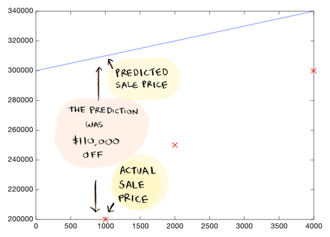
Maybe a drunk person drew this line...it is $110,000 dollars off the mark for that house. It is also far off all the other values:
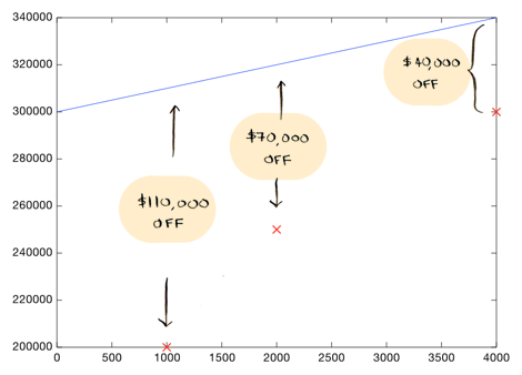
On average, this line is $73,333 off ($110,000 + $70,000 + $40,000 / 3).
Here's a better line:
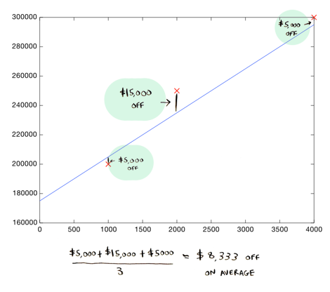
This line is an average of $8,333 dollars off...much better. This $8,333 is called the cost of using this line. The "cost" is how far off the line is from the real data. The best line is the one that is the least off from the real data. To find out what line is the best line, we need to use a cost function.
The cost function
First some foundational math. We are drawing a line. Here's what the equation of a line looks like:
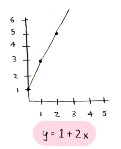
The first number tells you how high the line should be at the start:
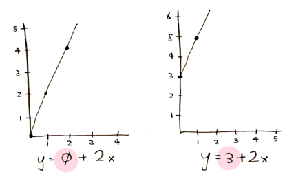
The second number tells you the angle of the line:
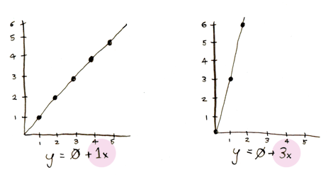
So we need to come up with two pretty good numbers that make the line fit the data. Here's how we do it:
- Pick two starting numbers. These are traditionally called
theta_0andtheta_1. Zero and zero are a good first guess for these. - Draw a line using those numbers:
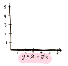
(Yes, it is a line where all the predicted values are zero. It is still a fine first guess, we are going to keep improving it).
- Calculate how far off we are, on average, from the actual data:
This is called the cost function. You pass theta_0 and theta_1 into the function, and it tells you how far off that line is (i.e. the cost of using that line).
I'll use Octave code, since that's what the course uses.
% x is a list of square feet: [1000, 2000, 4000]
% y is the corresponding prices for the homes: [200000, 250000, 300000]
function distance = cost(theta_0, theta_1, x, y)
  distance = 0
  for i = 1:length(x) % arrays in octave are indexed starting at 1
    square_feet = x(i)
    predicted_value = theta_0 + theta_1 * square_feet
    actual_value = y(i)
    % how far off was the predicted value (make sure you get the absolute value)?
    distance = distance + abs(actual_value - predicted_value)
  end
  % get how far off we were on average
  distance = distance / length(x)
end
I'll also show the math formula they use for this. It is pretty much the same thing:
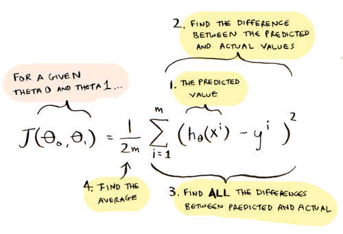
In this formula, h(x) represents the predicted value:
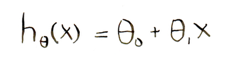
It's just the formula for our line! If we plug in a specific value for x, we will get a value for y.
So h(x) - y gives us the difference between the predicted value and the actual value.
For a given value of theta_0 and theta_1, the cost function will tell you how good those values are (i.e. it will tell you how far off your predictions were from the actual data). But what do we do based on that information? How do we find the values of theta_0 and theta_1 that will draw the best line? By using gradient descent.
Gradient descent

Let me start with a simpler version of gradient descent, and then move on to the real version. Suppose we decide to leave theta_0 at zero. So we experiment with what value theta_1 should be, but theta_0 is always zero. Now you can try various values for theta_1, and you will end up with different costs. You can plot all of these costs on a graph:
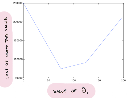
So for example, using a theta_1 value of 75 is better than a value of 160. The cost is lower:
Here are the corresponding lines (remember, theta_0 is zero in these lines):
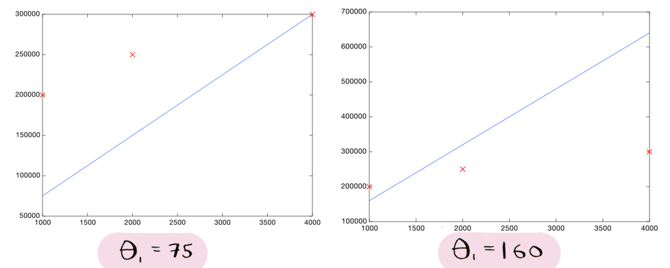
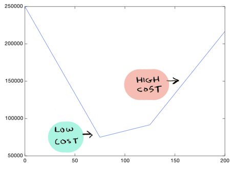
We can see that the line on the left seems to fit the data better than the line on the right, so it makes sense that the cost of that line is lower. And from this graph it looks like theta_1 = 75 gives us the lowest cost overall:
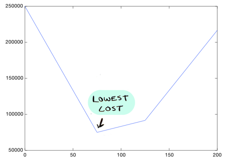
Since it is the lowest point in this graph. So with all the costs graphed out like this, we just need to find the lowest point on the graph, and that will give us the optimal value of theta_1!
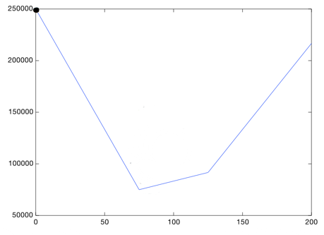
Gradient descent helps us find the lowest point on this graph. You start with a value for theta_1, and update it iteratively till you arrive at the best value. So you can start at theta_1 = 0. Then you have to ask, should I go left or right?
Well, we want to go down, so lets go right a small step:
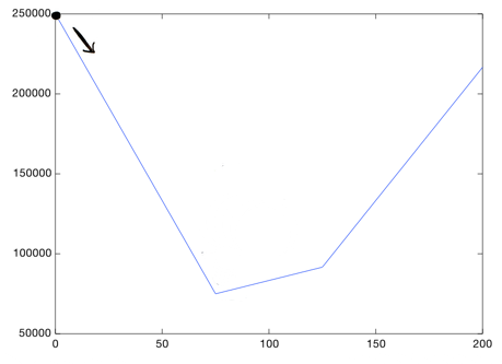
This is the new value for theta_1. Again we ask, should we go left or right? At each step, you need to head downward, till you get to a point where you're as low as you can go:
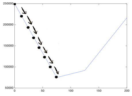
This is gradient descent: going down bit by bit till you hit the bottom. How do you figure out which way is down? The answer will be obvious to calculus experts but not so obvious for the rest of us: you take the derivative at that point. This is the part that I'll gloss over and just give you a formula to apply. But the important bit to know is, if you take the current value of theta_1 and add the derivative at that point, you will go down. You just do that a bunch of times (say 1000 times) and you will hit bottom!
That was the simpler view, now lets get back to the original problem. In this problem, we need to know the optimal values for both theta_0 and theta_1. So the graph looks more like this:
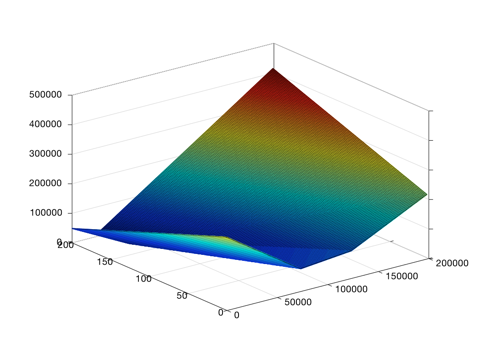
So you can see having theta_0 = 200000 and theta_1 = 200 would be really bad, but theta_0 = 100000 and theta_1 = 50 would be okay.
It is still a bowl with a low point, it is just in 3d because now we are considering theta_0 as well. But the idea stays the same: start somewhere in the bowl and just keep taking steps till you are at the bottom!
This is how you find the line with the lowest cost with gradient descent. You find the theta_0 and theta_1 values that give you the best fitting line by starting with a guess and incrementally updating that guess to make the cost lower and lower.
Here's the formula for gradient descent:
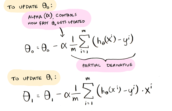
They are partial derivatives used in two update rules: one for theta_0 and another for theta_1. The two are almost the same, except the theta_1 derivative has that extra x at the end.
Putting it all together
The Octave code can be found here. Here's an R version thanks to Derek McLoughlin. Note: I used something called feature scaling here, so the square feet values will be [1, 2, 4] and not [1000, 2000, 4000] as expected. This just makes gradient descent work better here.
We started with these data points:
Using gradient descent, we find that theta_0 = 175000 and theta_1 = 32.143 give us the best fitting line, which costs $7,142.9 and looks like this:
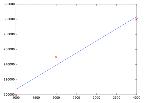
(our eyeballed line was really close, it had a cost of $8,333.33).
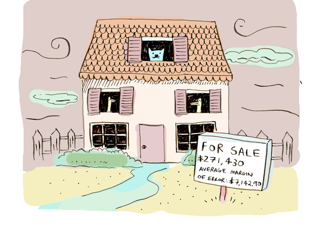
And know you know that you can sell your 3000 square foot home for $271,430 dollars!
One final note: Octave includes a function called fminunc that does the hard work of gradient descent for you...you just need to give it a cost function. Here's an example.
Read the followup to this post (logistic regression) here.
Recap
- Linear regression is used to predict a value (like the sale price of a house).
- Given a set of data, first try to fit a line to it.
- The cost function tells you how good your line is.
- You can use gradient descent to find the best line.
- Take the Coursera course here! It is great.